Skip to content
JG.Josh GutierrezGitHub

Josh Gutierrez / Investment research

Investment research.
Built for decisions.

I build constrained portfolios, test whether models add value, and turn corporate disclosures into traceable research. Start with the finding. Inspect the evidence.

Portfolio customization / historical result35.5% median reduction in tracking error.Minimum-risk versus proportional allocation · nine scenarios · net of modeled costs
MBA + MS in FinanceInstitutional perspective.
Independent research.
Abstract physical balance of sculptural forms, illustrating portfolio tradeoffs
01 / A study in tradeoffsConceptual illustration, not data

01 / Six featured projects

What the work delivers.
Why it matters.

Six projects, each led by a finding or a working capability. Explore the original exhibits, then open the evidence and implementation when you want more detail.

6 featured projects10 more

Jump to more projects
01 / Portfolio constructionHistorical study

The cost of customization

Finding

Trading about 60% less saved only $110 a year per $1 million, while adding 27 basis points of tracking error in the historical no-gold account.

Why it matters. Compare the dollar savings with the extra departure from the investment policy before choosing a lower-turnover allocation.

Historical eight-ETF study; assumed trading costs. Lower tracking risk is not higher return.

Three methods. One no-gold restriction.Original
What does less trading buy?Choose an allocation to compare.
Trading cost versus tracking risk in the no-gold accountOriginal study values, redrawn for comparison. Proportional: 1.7484% gross tracking error and 1.4154 basis points annual modeled cost. Minimum risk: 1.3691% and 1.8231 basis points. Lower turnover: 1.6390% and 0.7245 basis points. The highlighted point is the selected allocation. These are three discrete evaluated methods, not an estimated frontier.Annual modeled cost (bp)0121.21.41.61.8Gross tracking error (% / year)ProportionalMinimum riskLower turnover
Modeled cost / year$72at a constant $1m reference NAV
Gross tracking error1.64%annualized active-return variability

About $110 less cost. +27 bp tracking risk versus minimum risk.

Historical 2014–2025 study · Assumed costs · Gross tracking error is risk, not a fee or a predicted loss.
Explore the evidence

The result in context

Minimum-risk allocation reduced realized net tracking error by a median 35.5% across nine constrained scenarios versus bounded proportional allocation.

What I built

Compared three allocation methods across ten account scenarios in a 2014 to 2025 walk-forward simulation, using actual CRSP returns, lagged risk estimates, drifting holdings, and account-funded trading costs.

How to interpret it

A retrospective, fixed eight-ETF study with current-vintage data and assumed costs. Not live client outcomes, tax-aware advice, or evidence of alpha.

Method, checks & further questions
  1. 01

    Set the restriction

    Start with a policy allocation and an account constraint, such as no gold.

  2. 02

    Reconstruct and challenge

    Independently check the three allocation methods' accounting, timing, and constraints.

  3. 03

    Review the trade-off

    After the technical checks, compare tracking risk with modeled account costs.

The problem

A client can agree with an investment policy but be unable to hold one of its assets. Redistributing that asset's weight changes the portfolio's behavior. The question is how to honor the restriction while staying close to the plan, and whether fewer trades justify a larger departure.

What I built

The study compared three allocation methods across ten account scenarios from 2014 to 2025. A separately implemented Python + SQL checker reconstructed holdings, fees, account values, and return contributions across all 30 paths. It also checked that decisions preceded execution-day returns. Tracking error measures how variable portfolio-minus-policy returns are; it does not measure return-prediction skill.

The key decision

Separate the allocation engine from the accounting and timing checks: a plausible optimizer output still needs to be challenged. Deliberately inject faults, diagnose them, correct them, and retest before reviewing the investment trade-off. Then compare realized tracking risk with modeled dollar costs rather than assuming less turnover is always worth it.

What I learned

Minimum-risk allocation reduced realized tracking error by a median 35.5% across nine constrained scenarios. In the no-gold case, lower turnover saved about $110 a year per $1 million of reference account value versus minimum risk, while adding roughly 27 basis points of gross tracking error. Separately, 115 baseline controls passed and all five deliberately injected faults were blocked before a clean retest.

What I would test next

Extend the existing sensitivity work to alternative investment universes and evaluation periods before generalizing. The independent checker still shares source data and economic assumptions; it does not certify optimizer optimality.

Go one level deeper

  • What does an independent checker add, and which shared assumptions can it still miss?
  • When would $110 of modeled annual savings justify more tracking risk, and what could change that answer?
Results, methods & boundaries

Result. Minimum-risk allocation reduced realized net tracking error by a median 35.5% across nine constrained scenarios versus bounded proportional allocation.

Scope. A retrospective, fixed eight-ETF study with current-vintage data and assumed costs. Not live client outcomes, tax-aware advice, or evidence of alpha.

Implementation. Compared three allocation methods across ten account scenarios in a 2014 to 2025 walk-forward simulation, using actual CRSP returns, lagged risk estimates, drifting holdings, and account-funded trading costs.

  • WRDS / CRSP
  • CVXPY
  • Ledoit-Wolf
  • Walk-forward evaluation
Link to this project
Open the oversight labExplore the tax-lot transition labView research & codeExplore the scenarioRead the case studyDownload aggregate data
02 / Research toolsFrozen public prototype

Pure News Intelligence

Delivered capability

Trace 995 disclosure changes to their source passages, then inspect the evidence behind a research question.

Why it matters. An analyst can check what changed and what was already known before developing an investment thesis.

Frozen evidence demo, not live AI. Human usefulness review is still pending.

From source to research questionOriginal
KHC Kraft HeinzFrozen filing record
Prior 10-K · Feb 17, 2022
“…may increase the cost of financing as well as the risks of refinancing maturing debt.”
Current 10-K · Feb 16, 2023
“The creditors who hold our debt could accelerate amounts due in the event that we default…”
The analyst’s next question

What changed in covenant exposure or financing access?

A sourced example from the original disclosure-review workflow.
Explore the evidence

The result in context

995 evidence-backed disclosure changes. Eight bounded idea cases produced two hypotheses, six safe rejections, and zero actionable trade views.

What I built

An evidence-linked workflow that compares disclosures, checks prior context, preserves source spans, and challenges unsupported narratives before presenting a hypothesis.

How to interpret it

The demo serves frozen evidence packets, not live AI inference. Formal blinded human review and analyst-workflow validation remain pending.

Method, checks & further questions
  1. 01

    Find the change

    Compare consecutive disclosures and preserve the exact supporting passages.

  2. 02

    Check the context

    Look at earlier evidence and challenge the first interpretation.

  3. 03

    Question or reject

    Present a bounded research question, or explain why the idea did not survive.

The problem

A disclosure can sound important without containing genuinely new information. Analysts need to see what changed, what was already known, and which exact passages support an interpretation before spending time on a new thesis.

What I built

The workflow compares consecutive disclosures, links the changed text to source passages, checks earlier filings and eligible news, and separates facts from interpretations. A skeptical review searches for counterevidence before a research question is presented. The public demo displays frozen evidence packets.

The key decision

Keep change detection separate from hypothesis generation, and let the workflow reject weak ideas. A citation can support a factual statement without validating an investment thesis, so evidence coverage is not treated as proof of usefulness or trading value.

What I learned

The disclosure workflow produced 995 evidence-backed changes. A separate eight-case idea review retained two research hypotheses and rejected six cases; none became an actionable trade view. The demonstrated outcome is traceability and selective hypothesis formation, not proven analyst productivity.

What I would test next

Run blinded human review of the frozen packets before broader case evaluation or an analyst-workflow pilot.

Go one level deeper

  • What evidence should make the system reject an otherwise plausible idea?
  • How would you test analyst usefulness separately from citation accuracy?
Results, methods & boundaries

Result. 995 evidence-backed disclosure changes. Eight bounded idea cases produced two hypotheses, six safe rejections, and zero actionable trade views.

Scope. The demo serves frozen evidence packets, not live AI inference. Formal blinded human review and analyst-workflow validation remain pending.

Implementation. An evidence-linked workflow that compares disclosures, checks prior context, preserves source spans, and challenges unsupported narratives before presenting a hypothesis.

  • SEC filings
  • Evidence retrieval
  • Claim verification
  • Skeptical review
Link to this project
Open interactive demoView sourceWhy the research changed direction
03 / ML & deep learningApplied transformers · closed retrospective

When a language model meets trading costs

Finding

The generic sentiment strategy's Sharpe fell from 1.14 before costs to approximately zero after modeled base costs.

Why it matters. The appealing gross result did not justify promoting the strategy. Text interpretation and investable value need separate tests.

Pretrained Qwen and FinBERT inference; no transformer weights trained. Saved research results, not live predictions or validated alpha.

Applied transformers. Tested decisions.
Language is not an edge by itself.What survives the cost of acting on it?
QwenStructured assessment
FinBERTSentiment reference

Pretrained inference · no transformer weights trained

Five-session strategy · annualized SharpeNet
Generic sentiment0.0082
Event-surprise redesign-0.7014
Neither strategy was promoted.Base costs consumed the generic signal's apparent advantage. The redesign remained negative.
5,000 articles · 125 companiesChronological split: 3,000 development / 1,000 validation / 1,000 holdout
Inspect all six saved results
Five-session portfolio Sharpe by cost scenario
SpecificationGrossBase netHigher-cost net
Generic sentiment1.13960.0082-1.6210
Event-surprise redesign-0.2776-0.7014-1.1471

The redesign's holdout IC had been viewed before its portfolio specification was frozen. These are two related specifications, not independent replications. Cost controls reveal saved scenarios; they do not rerun models.

Download the aggregate comparison ↗
Saved historical NLP evaluation · Final redesign is a retrospective, not a pristine holdout · Modeled costs and licensed source data · No live inference or alpha claim.
Explore the evidence

The result in context

Generic sentiment's five-session Sharpe fell from 1.1396 gross to 0.0082 after base costs. The event-surprise redesign also failed its promotion gates. Neither was promoted as a trading strategy.

What I built

An evaluation pipeline for 5,000 articles using pretrained Qwen assessments and a FinBERT reference, typed outputs, immutable caches, chronological splits, outcome purging, and stateful portfolio accounting.

How to interpret it

Pretrained-model inference, not transformer training or fine-tuning. The final redesign followed previously viewed holdout IC; it is a retrospective, not a pristine confirmatory test. Licensed source data are not redistributed.

Method, checks & further questions
  1. 01

    Extract and compare

    Compare structured pretrained-model assessments with a finance-specific sentiment reference.

  2. 02

    Lock the evaluation

    Keep chronological splits, development-only calibration, and traceable cached inputs.

  3. 03

    Apply the decision rule

    Reconcile daily portfolio costs and uncertainty; close specifications that fail the gates.

The problem

Financial language can sound bullish without containing new, company-specific information. This project asks whether a structured model assessment improves on a finance-specific sentiment reference, then tests whether the resulting signal is useful after realistic portfolio constraints and modeled costs.

What I built

The frozen corpus contains 5,000 full-text articles for 125 companies, with chronological 3,000 / 1,000 / 1,000 development, validation, and holdout partitions. Pretrained Qwen supplies typed, cached assessments; pretrained FinBERT supplies a sentiment reference. The event-surprise signal combines their disagreement with specificity, materiality, novelty, and confidence. Edge calibration uses development observations only; split-crossing outcomes and overlapping same-company trades are excluded.

The key decision

Keep model-output validity separate from human-verified semantic accuracy, and event-level IC separate from portfolio Sharpe. Preserve the generic-sentiment result, then evaluate the narrower redesign against six predeclared promotion gates. Do not turn a failed retrospective into a success by tuning on its holdout.

What I learned

The generic five-session portfolio's Sharpe fell from 1.1396 before costs to 0.0082 with base costs and −1.6210 with conservative costs. The event-surprise redesign had a positive event-level rank IC of 0.0349, yet its 46 accepted holdout trades produced base-net Sharpe −0.7014 over 66 sessions. Three of six gates failed; the block-bootstrap 95% Sharpe interval was [−2.9615, 3.1299]. Neither specification was promoted.

What I would test next

For a future study, establish blinded human labels for specificity, novelty, and abstention; measure calibration against those labels; then freeze an untouched prospective evaluation. The existing redesign had already exposed holdout IC, and its modeled fills do not establish production execution quality.

Go one level deeper

  • Why can a positive event-level information coefficient coexist with a negative portfolio Sharpe?
  • How would you evaluate novelty and abstention without treating another model's answer as ground truth?
Results, methods & boundaries

Result. Generic sentiment's five-session Sharpe fell from 1.1396 gross to 0.0082 after base costs. The event-surprise redesign also failed its promotion gates. Neither was promoted as a trading strategy.

Scope. Pretrained-model inference, not transformer training or fine-tuning. The final redesign followed previously viewed holdout IC; it is a retrospective, not a pristine confirmatory test. Licensed source data are not redistributed.

Implementation. An evaluation pipeline for 5,000 articles using pretrained Qwen assessments and a FinBERT reference, typed outputs, immutable caches, chronological splits, outcome purging, and stateful portfolio accounting.

  • Qwen / FinBERT
  • Structured NLP
  • Purged time splits
  • Cost-aware evaluation
Link to this project
Explore the research & codeRead the frozen retrospectiveDownload cost comparisonRead methods & provenance
04 / Empirical researchCompleted forecasting study

When a simpler forecast is enough

Finding

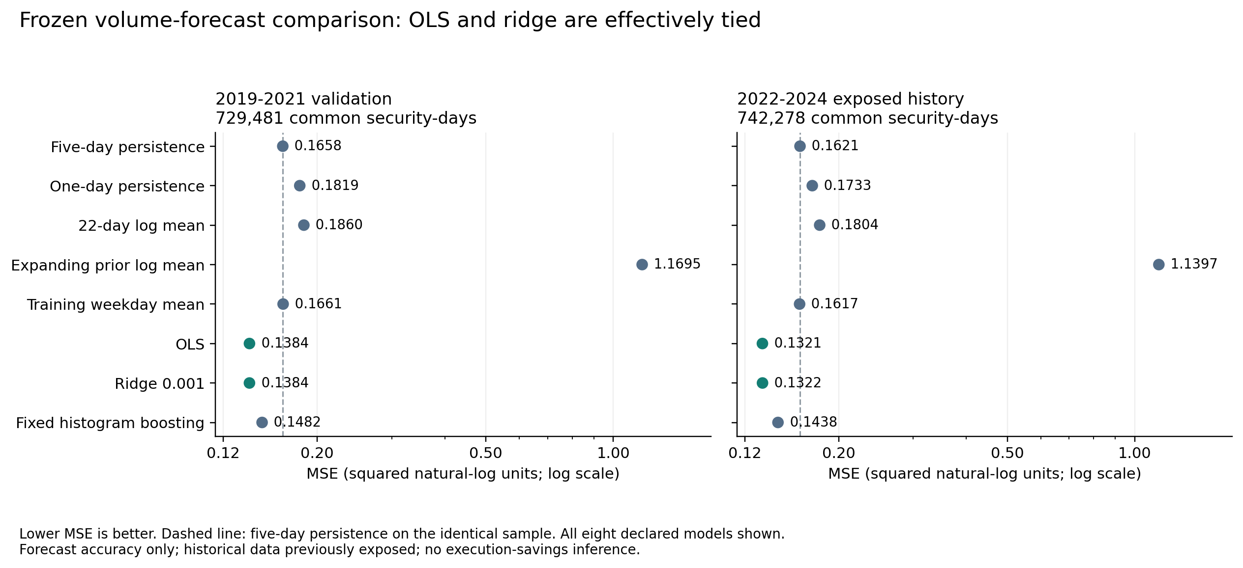
Ridge reduced validation forecast error by 16.6% versus persistence; ordinary least squares captured almost the same gain.

Why it matters. Keep the simpler linear model as the benchmark. More complex forecasting still has to demonstrate better execution decisions.

Completed forecast comparison; economic-value follow-up remains unfinished. Later historical data were previously exposed.

Forecasting is not execution.Original ↗
The linear model earns its place.Does extra complexity add anything?
16.6%

less forecast MSE with ridge
versus five-day persistence

2019–2021 validation · 729,481 common security-days
Mean squared forecast errorLower is better
Five-day persistence0.1658
OLS · simple linear0.1384
Ridge · regularized linear0.1384
Fixed histogram boosting0.1482
OLS ≈ ridge.Both beat fixed boosting. Regularization did not establish a meaningful gain over OLS.
Compare all 8 frozen methods
2019–2021 validation · same sample for every method
MethodMSEReduction vs baseline
Five-day persistence0.165837Baseline
One-day persistence0.181862-9.66%
22-day log mean0.185973-12.14%
Expanding prior log mean1.169494-605.21%
Training weekday mean0.166141-0.18%
OLS · simple linear0.13836816.56%
Ridge · regularized linear0.13835816.57%
Fixed histogram boosting0.14820210.63%

Negative reduction means worse than five-day persistence. MSE is measured in squared natural-log units.

Download both periods as CSV ↗
Saved historical forecast results · MSE in squared natural-log units · 2022–2024 previously exposed, not an untouched holdout · No demonstrated execution savings.
Explore the evidence

The result in context

Ridge reduced validation forecast MSE by 16.6% versus five-day persistence. Ordinary least squares captured essentially the same gain; fixed boosting did worse than both linear models.

What I built

Compared eight frozen volume-forecasting methods on identical security-days, with training-only estimation, lagged inputs, coverage accounting, and dependence-aware uncertainty.

How to interpret it

A restricted, current-vintage historical sample. The later 2022–2024 evaluation was previously exposed. Forecast accuracy is established within this study, not trading-cost savings or investment returns.

Method, checks & further questions
  1. 01

    Define the baseline

    Forecast activity relative to the prior five sessions, using only lagged information.

  2. 02

    Compare fairly

    Score all eight frozen methods on the same security-days and retain simple alternatives.

  3. 03

    Separate the decisions

    Choose a transparent forecasting baseline before testing economic value.

The problem

A portfolio team needs to think about how much can be traded, not just what to buy. Daily dollar volume is one useful activity proxy. This project first asks whether a forecast improves on simply carrying recent activity forward, before trying to connect that forecast to an execution decision.

What I built

The target is next-session log dollar volume relative to its prior five-session log average. Eight methods were compared on the same eligible observations: five simple baselines, OLS, ridge, and fixed histogram boosting. Fitting and scaling used 2010–2018 training data. Validation covered 729,481 security-days in 2019–2021. Frozen models were then replayed on 742,278 previously exposed security-days in 2022–2024, without refitting or reselection.

The key decision

Keep the easy-to-explain OLS model in the comparison, use identical samples, and retain every declared method. Otherwise, it is too easy to credit regularization or machine learning for gains that a simpler model already captures. Separate forecast error from economic value: a better volume forecast does not automatically mean cheaper execution.

What I learned

Ridge reduced forecast MSE by 16.6% in validation and 18.4% in the exposed historical evaluation versus five-day persistence. OLS was effectively tied, and fixed boosting was worse than both. The gain over persistence remained positive across the declared years, liquidity groups, and activity regimes. These checks support a useful forecasting baseline within this sample, not a trading-performance claim.

What I would test next

Evaluate the frozen simple models in a genuinely future or broader-universe sample. Establish corporate-action and settlement handling before a separately specified execution-cost comparison; that practical-value study is not complete.

Go one level deeper

  • Why might a lower log-volume forecast error fail to reduce execution costs?
  • What does OLS matching ridge change about which model you would put into an analyst workflow?
Results, methods & boundaries

Result. Ridge reduced validation forecast MSE by 16.6% versus five-day persistence. Ordinary least squares captured essentially the same gain; fixed boosting did worse than both linear models.

Scope. A restricted, current-vintage historical sample. The later 2022–2024 evaluation was previously exposed. Forecast accuracy is established within this study, not trading-cost savings or investment returns.

Implementation. Compared eight frozen volume-forecasting methods on identical security-days, with training-only estimation, lagged inputs, coverage accounting, and dependence-aware uncertainty.

  • WRDS / CRSP
  • OLS / ridge
  • Common-sample evaluation
  • Block bootstrap
Link to this project
Read the evidenceDownload model comparisonView the original chart
05 / Portfolio constructionResearch prototype

From analyst views to portfolio weights

Delivered capability

Turn analyst views and confidence assumptions into portfolio weights with explicit position, exposure and turnover limits.

Why it matters. Make the size of a proposed trade explainable—not just the conviction behind the recommendation.

Student-fund research prototype; no verified live deployment or performance improvement.

How a view becomes an allocationOriginal
Conviction is not a portfolio weight.Make the translation explicit.
  1. 01
    Start with a prior

    Factor-based expectations establish a reference.

  2. 02
    Blend views + confidence

    Black–Litterman incorporates analyst conviction.

  3. 03
    Constrain the allocation

    Optimization converts the blended inputs into portfolio weights.

What becomes reviewableThe path from a belief to a portfolio decision.
Conceptual workflow from the student-fund research prototype.
Explore the evidence

The result in context

A reviewable implementation connecting investment views to constrained allocations. No improved-performance claim is made.

What I built

A Black-Litterman implementation for student-fund research, combining factor-based priors, conviction-weighted views, constrained optimization, and portfolio attribution.

How to interpret it

A student-fund research prototype, not verified live deployment or evidence of improved investment performance.

Method, checks & further questions
  1. 01

    Start with a baseline

    Use factor-based expected returns as the starting assumptions.

  2. 02

    Add a view

    Blend analyst expectations according to explicit confidence assumptions.

  3. 03

    Apply the limits

    Find constrained weights and inspect their exposures and attribution.

The problem

An analyst's buy recommendation does not specify how large a position should be. A portfolio also has existing exposures, uncertain forecasts, position limits, and a finite trading budget. Those considerations need to meet in one reviewable process.

What I built

The Black-Litterman implementation starts with factor-based expected returns, blends in analyst views according to assumed confidence, and solves for allocations within portfolio constraints. Attribution then separates sector and factor contributions to help explain portfolio behavior.

The key decision

Represent conviction as uncertainty around a view rather than treating every forecast equally. Keep position, market-exposure, tracking-risk, and turnover constraints explicit, so the strongest individual view does not automatically dominate the portfolio.

What I learned

The implementation makes the path from prior assumptions to views to constrained weights inspectable. Confidence settings and constraints are part of the investment decision; the existence of an optimized allocation does not establish that its forecasts are accurate.

What I would test next

Evaluate how allocations change when confidence assumptions, expected returns, and constraints are perturbed, then compare against simpler allocation rules.

Go one level deeper

  • How should lowering confidence in a view change its effect on the portfolio?
  • How would you distinguish an allocation driven by a forecast from one driven by a binding constraint?
Results, methods & boundaries

Result. A reviewable implementation connecting investment views to constrained allocations. No improved-performance claim is made.

Scope. A student-fund research prototype, not verified live deployment or evidence of improved investment performance.

Implementation. A Black-Litterman implementation for student-fund research, combining factor-based priors, conviction-weighted views, constrained optimization, and portfolio attribution.

  • Black-Litterman
  • Factor attribution
  • CVXPY
  • Portfolio constraints
Link to this project
Explore the repository
06 / Research toolsResearch workbench

Optlab Research

Delivered capability

A reusable equity-research workbench connects ten registered signals and four universe presets to portfolio and cost reporting.

Why it matters. Inspect the universe, signal definition and accounting behind a result before interpreting its performance.

Archived 2023-12-29 signal diagnostic; synthetic software checks. Not a validated investment record.

Read the relationship, not the labelSource chart ↗
Do these signals tell the same story?Inspect four pairs from the original nine-signal matrix.
Book-to-marketGross profitability
Value / profitability: rank correlation -0.52Signed correlation on a scale from minus one to plus one. This measures cross-sectional co-movement in signal ranks, not return prediction.-1.0-0.50.00.51.0
-0.52rank correlation

Higher value ranks tended to coincide with lower profitability ranks in this saved cross-section.

Correlation between signals is not evidence that either predicts returns.

Archived liquid_500 cross-section · 2023-12-29 · Values transcribed at the source chart’s two-decimal precision; not freshly rerun.
Explore the evidence

The result in context

79 synthetic-fixture tests passed. The archived nine-signal cross-section exposes relationships worth investigating, not evidence of predictive returns.

What I built

A Python, DuckDB and Polars workbench separating data access, ten registered signals, four universe presets, portfolio construction and reporting. Packaged defaults and accounting paths are checked in Windows and Linux CI.

How to interpret it

Real-data runs require a separately prepared, licensed data lake. Universe presets are approximations; costs compare target weights, not drifting holdings. Archived notebook outputs have not been rerun after accounting repairs.

Method, checks & further questions
  1. 01

    Define the research inputs

    Choose a dated universe and signal specification with explicit data requirements.

  2. 02

    Inspect before combining

    Check distributions, coverage and cross-sectional relationships.

  3. 03

    Reconcile the result

    Separate gross returns, costs and net returns; preserve the run configuration.

The problem

An equity study can go wrong before its model runs: an inconsistent universe, unavailable fundamentals or a mischarged short trade can change the result. A research framework needs explicit contracts across those steps.

What I built

Separate universe SQL, a validated signal registry, cross-sectional calculations, portfolio construction and gross/net reporting. The public interfaces retain a caller-supplied universe, and accounting fixtures verify that both long and short transactions incur costs.

The key decision

Keep unsupported integrations and uncalibrated impact models explicit instead of letting their presence imply completed functionality. Preserve archived diagnostics while distinguishing them from freshly rerun results.

What I learned

The saved cross-section shows positive 0.14 rank correlation between momentum and reversal, despite an expectation of a negative relationship. Definitions, horizon and the sampled universe need inspection before interpreting a label.

What I would test next

Reconcile an end-to-end licensed-data run against an independent implementation, then test coverage, delisting treatment and cost sensitivity on matched samples.

Go one level deeper

  • Why is signal correlation not information coefficient?
  • What does a fundamentals-availability gate establish—and what does it leave unresolved?
  • Why must a short position's trading cost reduce, not increase, portfolio return?
Results, methods & boundaries

Result. 79 synthetic-fixture tests passed. The archived nine-signal cross-section exposes relationships worth investigating, not evidence of predictive returns.

Scope. Real-data runs require a separately prepared, licensed data lake. Universe presets are approximations; costs compare target weights, not drifting holdings. Archived notebook outputs have not been rerun after accounting repairs.

Implementation. A Python, DuckDB and Polars workbench separating data access, ten registered signals, four universe presets, portfolio construction and reporting. Packaged defaults and accounting paths are checked in Windows and Linux CI.

  • DuckDB
  • Polars
  • Signal registries
  • Transaction-cost accounting
Link to this project
Explore the workbenchRead the source notebook

More findings & tools

More projects / 10

Additional work in neural networks, real estate, credit risk, and more. Each summary tells you what the project contributes before you open it.

Empirical research · Completed null findingWhen more information does not helpAdding filing and news features did not establish incremental return-prediction value: the 95% interval for the IC change included zero.Explore
07 / Empirical researchCompleted null finding

When more information does not help

Finding

Adding filing and news features did not establish incremental return-prediction value: the 95% interval for the IC change included zero.

Why it matters. The evidence did not justify the added complexity for return prediction. Disclosure review is a separate use case to evaluate.

Completed null finding. Exact empirical reruns require licensed data.

A null result with a useful consequenceOriginal
Incremental information coefficient−0.00227
Not validated
The incremental IC interval includes zeroEstimate negative 0.00227. The 95% interval runs from negative 0.00567 to positive 0.00049. Because the interval includes zero, the study did not validate incremental return-predictive information.Zero−0.00567+0.0004995% interval · includes zero
Research decisionRetire the alpha hypothesis.
Build for investigation.
The study did not validate incremental alpha. That redirected the work toward evidence-linked analyst research.
Explore the evidence

The result in context

Incremental information coefficient: -0.00227, with a 95% interval of [-0.00567, 0.00049]. The study did not validate incremental alpha.

What I built

A point-in-time research design with locked comparisons, explicit stopping gates, and retained negative findings. The result informed the narrower Pure News analyst-workflow prototype.

How to interpret it

Public synthetic fixtures demonstrate pipeline behavior. Exact reproduction of the empirical estimates requires independently licensed data.

Method, checks & further questions
  1. 01

    Set the comparison

    Ask what annual filings and news add beyond the simpler specifications.

  2. 02

    Test incremental value

    Respect information timing and compare the locked results.

  3. 03

    Keep the finding

    Report the null result and separate the workflow opportunity from return prediction.

The problem

Adding annual filings and news makes a research pipeline more complex. That complexity is only justified for return prediction if the added information improves on simpler inputs, not merely if the final model has an attractive headline statistic.

What I built

The study compared added annual-filing and permitted-news features with existing current-report and control specifications. Comparisons were locked and inputs constrained by when information was available. The information coefficient, or IC, summarizes the relationship between a signal and subsequent returns; the key question was the improvement over the simpler comparison.

The key decision

Judge incremental value rather than the combined model's standalone score. Preserve the locked result and stopping rules when the added features do not help, instead of treating extra complexity as progress.

What I learned

The incremental IC was -0.00227, with a 95% interval of [-0.00567, 0.00049]. The interval includes zero and the study did not validate incremental alpha. This result informed the narrower Pure News workflow for evidence-linked disclosure review.

What I would test next

Evaluate the disclosure-review workflow on human usefulness. Any renewed return-prediction claim would need a separate, preregistered study with the required licensed data.

Go one level deeper

  • Why can a positive overall IC coexist with no incremental value from new features?
  • What should be frozen before testing a new signal, and what result would make you stop?
Results, methods & boundaries

Result. Incremental information coefficient: -0.00227, with a 95% interval of [-0.00567, 0.00049]. The study did not validate incremental alpha.

Scope. Public synthetic fixtures demonstrate pipeline behavior. Exact reproduction of the empirical estimates requires independently licensed data.

Implementation. A point-in-time research design with locked comparisons, explicit stopping gates, and retained negative findings. The result informed the narrower Pure News analyst-workflow prototype.

  • Point-in-time inputs
  • Locked comparisons
  • Null results
  • Reproducibility
Link to this project
Read the findingsView source
ML & deep learning · Probabilistic modeling prototypeMacro Regime HMMCompare a full-history regime description with states estimated sequentially, using only observations available to the model at each step.Explore
08 / ML & deep learningProbabilistic modeling prototype

Macro Regime HMM

Delivered capability

Compare a full-history regime description with states estimated sequentially, using only observations available to the model at each step.

Why it matters. See where hindsight changes the story before using a regime label in an allocation experiment.

Synthetic 2000–2024 demonstration. State names describe fitted yield-curve ordering, not verified economic regimes.

What did the model know at the time?Source chart ↗
Hindsight and filtering are different tasks.Compare the same months under two information sets.

Full historyIncludes observations through 2024

  1. JanHigh slope
  2. FebHigh slope
  3. MarHigh slope
  4. AprHigh slope
  5. MayHigh slope
  6. JunHigh slope
  7. JulHigh slope
  8. AugHigh slope
  9. SepHigh slope
  10. OctHigh slope
  11. NovHigh slope
  12. DecHigh slope

Sequential filteringParameters fitted before each month

  1. JanHigh slope
  2. FebHigh slope
  3. MarMiddle slope
  4. AprHigh slope
  5. MayHigh slope
  6. JunHigh slope
  7. JulHigh slope
  8. AugHigh slope
  9. SepMiddle slope
  10. OctHigh slope
  11. NovHigh slope
  12. DecHigh slope
H / High slopeM / Middle slopeL / Low slope
2of 12 states differ

Differences can reflect future information, refitted parameters and changing state boundaries—not necessarily errors.

Only the filtered state enters the allocation experiment, and only in the following calendar month.

Synthetic 2000–2024 series · Seed 42 · First 60 months train the model. State labels follow fitted yield-curve means, not verified recession categories.
Explore the evidence

The result in context

45 tests passed, including exhaustive state-path calculations, future-perturbation checks and hand-calculated timing/cost examples. The 300-month synthetic demonstration produces 240 filtered states and 239 lagged proxy returns.

What I built

An inspectable Gaussian hidden Markov model with Baum–Welch estimation, Viterbi decoding, smoothing and chronological filtering. Training-only scaling and a one-calendar-month allocation lag separate retrospective diagnostics from a factor-exposure experiment.

How to interpret it

This is a classical probabilistic model, not a neural network. Synthetic states are not NBER recessions; current-vintage online data are not point-in-time history. The allocation proxy is not a tradable portfolio or evidence of alpha.

Method, checks & further questions
  1. 01

    Fit on prior observations

    Estimate the scaler and Gaussian HMM strictly before the classified month.

  2. 02

    Filter the observed prefix

    Retain transition history without using future observations.

  3. 03

    Apply a calendar lag

    The month-end state can first affect the next month's factor exposure.

The problem

A model that sees the entire history can use future observations to label the past. That is useful for description, but it cannot justify allocating with information that was unavailable at the time.

What I built

Implement Gaussian emissions, forward–backward inference and Viterbi decoding, then keep a distinct chronological path. At each refit, fit scaling and parameters on prior months only; filter through the current month and use its state no earlier than the next month.

The key decision

Label states by high, middle or low fitted yield-curve mean instead of treating them as established expansion or recession probabilities. Keep full-sample diagnostics out of the allocation inputs.

What I learned

The source-based exhibit lets you compare the two paths directly. Differences can reflect future information, parameter refits and state-boundary changes; they are not automatically classification errors.

What I would test next

Validate release-time and revision assumptions with a true vintage dataset, compare multiple initializations and simpler state rules, and preregister a genuinely untouched evaluation.

Go one level deeper

  • How do filtering, smoothing and Viterbi decoding differ?
  • Why does a chronological split still fail to reconstruct revised macro data?
  • What information belongs in the trade decision at month-end?
Results, methods & boundaries

Result. 45 tests passed, including exhaustive state-path calculations, future-perturbation checks and hand-calculated timing/cost examples. The 300-month synthetic demonstration produces 240 filtered states and 239 lagged proxy returns.

Scope. This is a classical probabilistic model, not a neural network. Synthetic states are not NBER recessions; current-vintage online data are not point-in-time history. The allocation proxy is not a tradable portfolio or evidence of alpha.

Implementation. An inspectable Gaussian hidden Markov model with Baum–Welch estimation, Viterbi decoding, smoothing and chronological filtering. Training-only scaling and a one-calendar-month allocation lag separate retrospective diagnostics from a factor-exposure experiment.

  • Gaussian HMM
  • Forward filtering
  • Baum–Welch EM
  • Chronological evaluation
Link to this project
Explore the modelInspect the timing contractDownload exhibit data
Portfolio construction · Synthetic allocation studyEqual capital is not equal riskIn the simulated ten-ETF portfolio, unequal capital weights balance modeled risk contributions at approximately 10% per asset.Explore
09 / Portfolio constructionSynthetic allocation study

Equal capital is not equal risk

Finding

In the simulated ten-ETF portfolio, unequal capital weights balance modeled risk contributions at approximately 10% per asset.

Why it matters. Evaluate diversification in risk contributions as well as dollars invested.

Seeded ten-ETF simulation. The displayed date is a simulation label, not observed market performance.

Same snapshot. Two ways to see the portfolio.Source chart ↗
Capital weight ≠ risk share.Change the portfolio, then compare the two views.
Equal risk contribution: capital weightsDBC: 4.55 percent. EEM: 4.79 percent. EFA: 4.01 percent. EMB: 17.01 percent. GLD: 5.18 percent. SHY: 18.59 percent. SPY: 6.38 percent. TIP: 16.10 percent. TLT: 18.68 percent. VNQ: 4.70 percent. Solid reference: zero. Dashed reference: ten percent per asset. Negative contributions extend left of zero.0%10%DBC4.6%EEM4.8%EFA4.0%EMB17.0%GLD5.2%SHY18.6%SPY6.4%TIP16.1%TLT18.7%VNQ4.7%

ERC balances modeled risk contributions, not dollars invested.

Exact snapshot values
Equal risk contribution · synthetic snapshot
AssetCapitalRisk share
DBC4.555%10.000%
EEM4.787%10.000%
EFA4.012%10.000%
EMB17.013%10.000%
GLD5.179%10.000%
SHY18.586%10.000%
SPY6.384%10.000%
TIP16.101%10.000%
TLT18.683%10.000%
VNQ4.701%10.000%
Synthetic ten-ETF snapshot · 2024-06-26 · Full-covariance risk shares are estimates, not forecasts of losses.
Explore the evidence

The result in context

In the seeded demonstration, unequal capital weights target approximately 10% of portfolio variance per asset. Eighteen tests check optimization, timing, covariance and holdings accounting.

What I built

A ten-ETF allocation prototype connecting SciPy equal-risk-contribution optimization to DuckDB covariance estimates and drifting-holdings accounting, with inverse-volatility, equal-weight and 60/40 comparators.

How to interpret it

The exhibit uses simulated prices. The model excludes trading costs, taxes, financing and leverage; it does not establish real-market outperformance.

Method, checks & further questions
  1. 01

    Estimate covariance

    Measure trailing variation and co-movement on a complete price panel.

  2. 02

    Allocate by risk

    Solve for equal variance contributions, then compare simple allocations.

  3. 03

    Track actual holdings

    Let weights drift between rebalances and check the resulting NAV independently.

The problem

A high-volatility holding can dominate portfolio risk even at a modest capital weight. Correlations matter too: inverse volatility ignores how an asset moves with the rest of the portfolio.

What I built

Estimate trailing covariance, solve for equal contributions to portfolio variance, and compare the result with inverse-volatility and equal-weight allocations. SQL tracks holdings drift and applies targets only after their decision date.

The key decision

Show capital and risk side by side, and retain simple comparators. The optimizer is only useful if the covariance inputs and subsequent holdings arithmetic are correct.

What I learned

The synthetic snapshot makes the distinction tangible: the equal-risk allocation can look uneven in dollars while its modeled risk contributions are almost equal. That balance is an ex-ante property, not a promise about future losses.

What I would test next

Evaluate robust covariance choices and realistic implementation costs on permitted historical data, with point-in-time availability and matched baselines.

Go one level deeper

  • When do inverse volatility and equal risk contribution agree?
  • How can correlations change risk shares without changing capital weights?
  • Why should the return on the decision date not be earned by the newly computed target?
Results, methods & boundaries

Result. In the seeded demonstration, unequal capital weights target approximately 10% of portfolio variance per asset. Eighteen tests check optimization, timing, covariance and holdings accounting.

Scope. The exhibit uses simulated prices. The model excludes trading costs, taxes, financing and leverage; it does not establish real-market outperformance.

Implementation. A ten-ETF allocation prototype connecting SciPy equal-risk-contribution optimization to DuckDB covariance estimates and drifting-holdings accounting, with inverse-volatility, equal-weight and 60/40 comparators.

  • Equal risk contribution
  • SciPy SLSQP
  • Rolling covariance
  • DuckDB SQL
Link to this project
Explore the researchRead the methodologyDownload exhibit data
ML & deep learning · Historical walk-forward studyA high R² is not a winning forecastUsing last month's housing index had roughly half the random forest's forecast error: RMSE 2.78 versus 5.58 index points.Explore
10 / ML & deep learningHistorical walk-forward study

A high R² is not a winning forecast

Finding

Using last month's housing index had roughly half the random forest's forecast error: RMSE 2.78 versus 5.58 index points.

Why it matters. The forest's high R² was not a reason to replace the simpler forecast in this historical comparison.

61 historical evaluation months · Macro release timing not controlled · Archived evaluated source included.

Tree ensembles / Test the benchmarkOriginal ↗
Good fit. Wrong benchmark?Switch from the index level to the errors it hides.
Random-forest R²0.978
RMSE / index points5.58 vs 2.78Forest vs last month's value · lower is better
Forest — dashedLag-one — dotted
Absolute prediction errors, January 2020 to January 2025Saved monthly historical results. Forest root mean squared error 5.579 index points; lag-one baseline 2.782. Select a month below for exact values. Historical macro inputs are not release-date controlled.Absolute error / index points0481220202022–232025

May 2022 · absolute errorForest 8.52 / Lag-one 2.73

A smaller error is better. Both methods use the same target month.

100 trees14 features61 refits
Historical archived evaluation · Current-vintage macro inputs, not a real-time information set · Original predictions redrawn, not new model output.
Explore the evidence

The result in context

Random-forest R² was 0.978, but RMSE was 5.58 index points versus 2.78 for lag-one persistence: about twice the error.

What I built

A 100-tree scikit-learn ensemble with 14 inputs, expanding-window monthly refits, fixed seed, saved predictions, and a matched lag-one benchmark across 61 evaluation months.

How to interpret it

Historical, current-vintage data with contemporaneous macro inputs. Release timing and revisions are not controlled; this is not a real-time forecasting result. The archived evaluation snapshot is supplied separately from the original notebook repository.

Method, checks & further questions
  1. 01

    Build the information set

    Combine ten macro series and four index lags; distinguish observation dates from release dates.

  2. 02

    Refit in calendar order

    Fit a fresh 100-tree ensemble on prior rows for each evaluation month.

  3. 03

    Challenge the score

    Compare saved errors with persistence on the same 61 observations.

The problem

A slowly changing housing index is an easy place to mistake a high R² for a useful forecast. A model can trace the broad trend while still predicting the next observation less accurately than persistence. The benchmark has to reflect what the model would replace.

What I built

The model uses scikit-learn's RandomForestRegressor: 100 trees, seed 42, ten macroeconomic inputs and index lags of 1, 3, 6 and 12 months. At each month from January 2020 to January 2025, a fresh forest is fitted only on earlier rows. Actual values, forest predictions and the lag-one baseline are saved for all 61 months. The portfolio exhibit redraws that original comparison and adds an error view; it does not retrain the model in the browser.

The key decision

Score the same observations against a simple lag-one forecast, not just against the overall sample mean implicit in R². Keep calendar-order fitting separate from point-in-time data availability: restricting training rows is necessary, but contemporaneous revised macro data can still make a backtest unrealistic.

What I learned

R² reached 0.978, but random-forest RMSE was 5.579 versus 2.782 index points for persistence. The current specification fails its baseline. This supports rejecting the model as a forecasting improvement; it does not prove that all tree models fail on housing or explain the entire error pattern.

What I would test next

Build a release-date-aware, vintage-data panel. Evaluate changes rather than only index levels, tune on nested chronological validation windows, compare with linear and persistence baselines, and freeze a future evaluation period. These are proposed next tests, not completed results.

Go one level deeper

  • Why can a model have high R² and still lose badly to a naive forecast?
  • How would release delays, revisions, and tree extrapolation affect the next experiment?
Results, methods & boundaries

Result. Random-forest R² was 0.978, but RMSE was 5.58 index points versus 2.78 for lag-one persistence: about twice the error.

Scope. Historical, current-vintage data with contemporaneous macro inputs. Release timing and revisions are not controlled; this is not a real-time forecasting result. The archived evaluation snapshot is supplied separately from the original notebook repository.

Implementation. A 100-tree scikit-learn ensemble with 14 inputs, expanding-window monthly refits, fixed seed, saved predictions, and a matched lag-one benchmark across 61 evaluation months.

  • scikit-learn
  • Random forest
  • Expanding-window refits
  • Baseline comparison
Link to this project
Read the evaluationDownload predictionsDownload evaluated sourceOriginal notebook repository
Risk & underwriting · Scenario simulationWhen does a loan breach its covenants?Under the simulated loan terms, 43.5% of paths breached a covenant by year one; 89.8% had breached by year five.Explore
11 / Risk & underwritingScenario simulation

When does a loan breach its covenants?

Finding

Under the simulated loan terms, 43.5% of paths breached a covenant by year one; 89.8% had breached by year five.

Why it matters. Review covenant headroom throughout the loan's life, not only at maturity. A breach is not the same as a default.

200,000 simulated paths, seed 42. Covenant breach is not default; probabilities depend on the stated case assumptions.

Follow the loan through timeOriginal ↗
A loan has to pass along the way.Choose a horizon in the original simulation.
Cumulative covenant-breach probabilityIn 200,000 simulated paths, at least one covenant breach occurred in 43.5 percent by year one, 70.9 percent by year two, 82.8 percent by year three, 87.5 percent by year four, and 89.8 percent by year five. The selected horizon is year 5, at 89.8 percent. These conditional probabilities are not default probabilities.Paths with a breach by this point (%)05010012345Years into the loan
89.8%

of simulated paths with at least one breach by year 5

Year-5 end loan tests

DSCR ≥ 1.200x
Debt yield ≥ 7.500%

Longer horizons include earlier breaches. Requirements also tighten; this is not a forecast of when a borrower defaults.

200,000 simulated paths · Seed 42 · Assumption-sensitive case study. Assumptions & evidence ↗
Explore the evidence

The result in context

Under the case-study assumptions, 43.5% of simulated paths breached at least one covenant by year one, rising to 89.8% by year five.

What I built

A seeded, 200,000-path Monte Carlo model of a five-year senior/mezzanine capital stack, combining mean-reverting rates, uncertain operating income, and quarterly covenant tests.

How to interpret it

Assumption-sensitive simulation, not observed loan performance or default probability. Rates and operating income are independent; refinancing, cures, waivers, and principal repayments are not modeled.

Method, checks & further questions
  1. 01

    Define the loan tests

    Specify the debt structure and the coverage and debt-yield requirements each quarter.

  2. 02

    Simulate the paths

    Move rates and operating income through 200,000 seeded five-year scenarios.

  3. 03

    Locate the pressure

    Compare breach risk across horizons and identify assumptions that need underwriting review.

The problem

A lender does not only care about a property's cash flow at the end of a holding period. The loan can require interest coverage and a minimum income-to-debt ratio each quarter. Rising borrowing costs or tighter requirements can create a breach even before maturity.

What I built

The model simulates five years of mean-reverting SOFR and uncertain net operating income for a fixed senior/mezzanine capital stack. Each quarter it checks debt-service coverage, or DSCR, and debt yield. DSCR compares income with interest due; debt yield compares annual income with the outstanding loan balance. A seeded, vectorized implementation makes the scenario reproducible.

The key decision

Measure whether a covenant was breached at any point, not only whether the final quarter passed. Keep the two loan tests separate, and distinguish a contractual breach from a default: a real loan may have cure rights, waivers, or other remedies that this model does not include.

What I learned

In the 200,000-path case, the share with at least one breach rose from 43.452% by year one to 89.758% by year five. The median maturity DSCR was 1.179x against a 1.20x floor. These results identify assumptions and covenant headroom to challenge; they do not estimate a real borrower's default probability.

What I would test next

Calibrate income, interest-rate exposure, and their dependence to authorized property and loan records. Then test actual amortization, hedges, refinancing, cure rights, and alternative covenant schedules before using the model for a lending decision.

Go one level deeper

  • Why can a loan pass at maturity but still have breached a covenant earlier?
  • Which matters more for this case: rates, operating income, or the tightening covenant schedule—and how would you test it?
Results, methods & boundaries

Result. Under the case-study assumptions, 43.5% of simulated paths breached at least one covenant by year one, rising to 89.8% by year five.

Scope. Assumption-sensitive simulation, not observed loan performance or default probability. Rates and operating income are independent; refinancing, cures, waivers, and principal repayments are not modeled.

Implementation. A seeded, 200,000-path Monte Carlo model of a five-year senior/mezzanine capital stack, combining mean-reverting rates, uncertain operating income, and quarterly covenant tests.

  • Monte Carlo
  • Debt covenants
  • Cash-flow stress
  • Seeded simulation
Link to this project
View the original case & notebookRead assumptions & evidenceDownload aggregate results
Empirical research · Synthetic benchmarkMapping competitive crowdingA six-dimensional business-model map recovered relative crowding with a 0.32 rank correlation in a synthetic benchmark.Explore
12 / Empirical researchSynthetic benchmark

Mapping competitive crowding

Finding

A six-dimensional business-model map recovered relative crowding with a 0.32 rank correlation in a synthetic benchmark.

Why it matters. The result supports a measurement pilot—not a stock-selection claim—before testing the map on real companies.

Synthetic measurement benchmark only; no real-company validation.

Can we measure competitive crowding?Original
Crowding recoveryρ = 0.3215

Separate measurement result
Synthetic · pooled Spearman

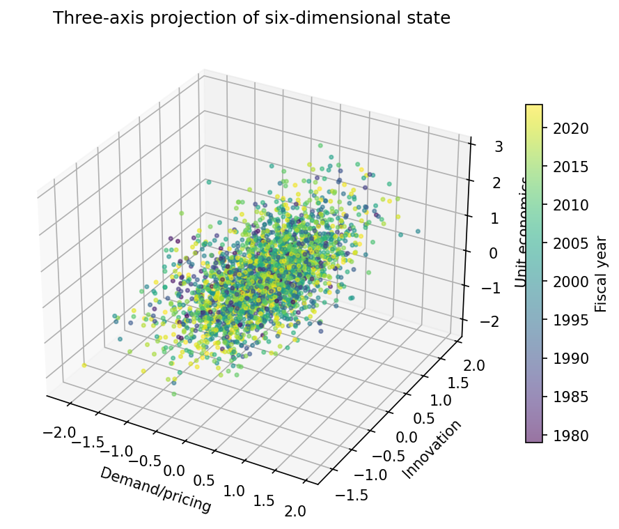
Original three-axis projection of the six-dimensional synthetic business-model state: demand and pricing, innovation, and unit economics, colored by fiscal year. Nearby synthetic observations occupy similar positions on these dimensions.
6 dimensions in the model3 shown in this projection
Original three-axis projection of the synthetic benchmark, colored by fiscal year.
Explore the evidence

The result in context

The crowding measure recovered latent density with pooled Spearman correlation 0.3215 in the synthetic benchmark.

What I built

A six-dimensional representation with time-aware transformations and separate, preregistered tests of measurement, survival, and portfolio utility.

How to interpret it

No real-company validation. Return, general-survival, and stable-taxonomy claims were rejected; the result is measurement-only.

Method, checks & further questions
  1. 01

    Represent the firm

    Describe business economics with six consistently oriented dimensions.

  2. 02

    Measure crowding

    Compare nearby positions using information available at each date.

  3. 03

    Test each claim

    Check measurement, prediction, and portfolio utility separately.

The problem

Companies in the same industry can have very different economics, while companies in different industries can share important characteristics. This project asks whether a structured business-model map can measure how crowded a firm's position is before asking whether that matters for investment outcomes.

What I built

The framework represents firms along six dimensions, including pricing power, defensibility, innovation, and capital efficiency. It uses time-aware transformations and synthetic scenarios with known underlying structure to test whether nearby points actually recover competitive crowding. Predictive and investment claims are evaluated separately.

The key decision

Separate measurement from prediction. Recovering a known pattern in a synthetic world can support a measurement method, but it cannot establish real-company relevance, survival prediction, or profitable trading.

What I learned

The crowding measure achieved a pooled rank correlation of 0.3215 with the synthetic world's underlying density. General survival, investable-return, and stable-taxonomy claims were rejected. The surviving result is a candidate measurement architecture for further research.

What I would test next

Begin a measurement-only real-company pilot: freeze the inputs, check coverage and stability without opening outcomes, then seek blinded analyst review before testing prediction.

Go one level deeper

  • What can synthetic recovery establish, and what still requires real-company evidence?
  • How would you test whether the map is stable without selecting it for attractive returns?
Results, methods & boundaries

Result. The crowding measure recovered latent density with pooled Spearman correlation 0.3215 in the synthetic benchmark.

Scope. No real-company validation. Return, general-survival, and stable-taxonomy claims were rejected; the result is measurement-only.

Implementation. A six-dimensional representation with time-aware transformations and separate, preregistered tests of measurement, survival, and portfolio utility.

  • Representation design
  • Temporal validation
  • Synthetic recovery
  • Claim ledger
Link to this project
Read the research
Risk & underwriting · Volatility-model mechanicsWhen bad news changes the riskWith the illustrated parameters, a −2% shock gives GJR 22.61% annualized volatility versus 20.26% after a +2% shock; GARCH treats both alike.Explore
13 / Risk & underwritingVolatility-model mechanics

When bad news changes the risk

Finding

With the illustrated parameters, a −2% shock gives GJR 22.61% annualized volatility versus 20.26% after a +2% shock; GARCH treats both alike.

Why it matters. A risk model's treatment of negative shocks is an explicit choice you can inspect before comparing forecasts.

Illustrative parameters and hand-checked recursions. No fitted market result, strategy return, or validated forecast ranking.

A model assumption you can inspectSource chart ↗
Same-sized shock. Different risk response.Move between a gain and an equal-sized loss.
Next-session annualized volatility after a -2% innovationGARCH 21.47 percent; GJR 22.61 percent. Both curves use illustrative parameters. The horizontal reference is prior annualized volatility of 20 percent, not a risk limit.15%20%25%30%35%40%-5% shock0% shock+5% shock
GARCH · solid blue21.47%Symmetric response
GJR · dashed red22.61%Sign-sensitive response

Annualized conditional volatility, not a predicted loss. These fixed parameters illustrate the mechanism; they do not establish forecast accuracy.

Adapted from the project’s original news-impact equations · Illustrative parameters · Prior annualized volatility 20%, 252 sessions per year.
Explore the evidence

The result in context

The 41-scenario exhibit and four independent arithmetic checks show exactly how the GJR negative-shock term changes conditional variance. This is a mechanism demonstration, not an empirical model ranking.

What I built

A from-scratch volatility-modeling project spanning GARCH, GJR-GARCH, EGARCH and HAR-RV. This bounded exhibit develops the original news-impact comparison, isolating the symmetric GARCH and asymmetric GJR recursions at explicit parameters.

How to interpret it

Parameters are illustrative, not estimated. Full-pipeline convergence, forecast comparison and VaR coverage require separate validation; no legacy performance ranking is presented as verified evidence.

Method, checks & further questions
  1. 01

    Fix the starting state

    Use the same prior variance and explicit, illustrative model parameters.

  2. 02

    Change one innovation

    Compare equal positive and negative shocks without refitting.

  3. 03

    Separate mechanism from evidence

    Check the arithmetic, then require a separate empirical forecast comparison.

The problem

Risk often clusters, and negative equity returns can be followed by a different volatility response than equally large gains. A constant risk estimate misses clustering; a symmetric model cannot express this sign effect.

What I built

The original project implements Gaussian likelihood estimation and several conditional-volatility models. The exhibit isolates two news-impact equations, holds prior volatility and parameters fixed, and varies only the observed return innovation.

The key decision

Separate explaining a model's mechanism from establishing its forecasting value. A plausible asymmetric curve still needs a fair held-out comparison against symmetric and simple volatility baselines.

What I learned

Adding a negative-shock coefficient changes the next variance forecast mechanically. It does not establish that the coefficient is stable, that the model is correctly calibrated, or that a larger estimated risk improves an investment decision.

What I would test next

Validate full-pipeline estimation and forecast timing, align all models to the same realized-variance proxy and test dates, and evaluate VaR coverage separately from forecast loss.

Go one level deeper

  • Why is volatility not a loss threshold?
  • What does a positive GJR gamma change, holding other parameters fixed?
  • Why must all forecast models use the same target and evaluation dates?
Results, methods & boundaries

Result. The 41-scenario exhibit and four independent arithmetic checks show exactly how the GJR negative-shock term changes conditional variance. This is a mechanism demonstration, not an empirical model ranking.

Scope. Parameters are illustrative, not estimated. Full-pipeline convergence, forecast comparison and VaR coverage require separate validation; no legacy performance ranking is presented as verified evidence.

Implementation. A from-scratch volatility-modeling project spanning GARCH, GJR-GARCH, EGARCH and HAR-RV. This bounded exhibit develops the original news-impact comparison, isolating the symmetric GARCH and asymmetric GJR recursions at explicit parameters.

  • Conditional variance
  • GARCH / GJR
  • News-impact curves
  • Model interpretation
Link to this project
Inspect the model projectRead the exhibit methodologyDownload exhibit data
ML & deep learning · Audited synthetic research prototypeLearning positions, not price targetsA trained PyTorch LSTM maps 63-day feature sequences to bounded positions, with inspectable sizing and portfolio accounting.Explore
14 / ML & deep learningAudited synthetic research prototype

Learning positions, not price targets

Delivered capability

A trained PyTorch LSTM maps 63-day feature sequences to bounded positions, with inspectable sizing and portfolio accounting.

Why it matters. The synthetic demonstration makes the signal-to-position pipeline inspectable; it does not establish market skill. Its training-cost alignment still needs repair.

Archived audited source and seeded synthetic results are downloadable. The original public repository is a different, earlier version; its advertised market returns are not used here.

Synthetic execution evidence onlyOriginal ↗
Learn a position. Inspect every fold.PyTorch LSTM · risk-aware objective · nine test folds
Maximum drawdown (%)Saved synthetic run
Maximum drawdown (%) across nine synthetic walk-forward foldsFold 6 is selected: -8.19 percent. Use the buttons below to inspect each fold. Full values are in the accessible data table.-10-50012345678
Select a recorded fold
-8.19%

Fold 6 · maximum drawdown
Largest peak-to-trough decline within this fold.

Inside the trained network
  1. 63 days × 14 featuresVolatility-scaled returns, MACD, breakouts, and moving-average distances.
  2. LSTM · 8 hidden unitsThe saved compact run learns a sequence representation; the full configuration uses 32 units.
  3. Dense → ReLU → dropout → tanhAn 8-unit head produces a bounded signal, then volatility scaling and a portfolio leverage cap size positions.
  4. Train → validate → testA Sharpe-style objective, Adam, gradient clipping, and validation-based checkpoint selection precede each unseen synthetic test slice.

The engineering lesson is to inspect the loss, execution timing, and every fold—not infer market skill from a neural-network label. Read the audit and remaining tests ↗

Read all nine fold records
Archived synthetic run · values in percent
FoldAnn. returnVolatilityMax. drawdown
01.036.24-3.66
1192.9113.75-2.78
243.0212.39-2.99
3-8.077.81-3.90
43.924.59-3.51
520.7013.59-6.39
61.5311.53-8.19
7-16.254.17-4.82
8173.0217.37-3.36
Download original fold records ↗
A working deep-learning research pipeline, not validated trading alpha. Simulated ETF-like data · 5 bps turnover costs · no real-market benchmark established. Architecture and figures refer to the archived audited version.
Explore the evidence

The result in context

An archived seeded run completed nine synthetic walk-forward folds. The exhibit exposes every fold and the actual network architecture, including unstable outcomes that a single average would hide.

What I built

A PyTorch LSTM with 14 volatility-scaled features, a differentiable Sharpe-style objective, bounded position outputs, validation-based checkpoints, gradient clipping, and walk-forward evaluation with realized turnover costs.

How to interpret it

Synthetic execution evidence only, not historical alpha. The training turnover proxy uses shuffled batches; the archived Sharpe field is CAGR divided by volatility. A chronological objective and real-market baseline study remain open.

Method, checks & further questions
  1. 01

    Represent the sequence

    Encode volatility-scaled features with an LSTM and emit a bounded position signal.

  2. 02

    Align learning and execution

    Inspect how the objective, sizing, signal dates, and realized costs relate.

  3. 03

    Inspect all outcomes

    Keep every synthetic test fold visible before designing a market-data baseline comparison.

The problem

A price forecast does not specify how large a position to take. This research implementation explores the Deep Momentum Network idea from Lim, Zohren, and Roberts: learn a bounded signal from a time sequence and optimize a risk-adjusted objective directly. The useful technical question is whether the network, loss, and execution accounting describe the same decision.

What I built

The saved compact run uses 63-day sequences of 14 engineered features, an eight-unit PyTorch LSTM, an eight-unit dense head with ReLU and dropout, and a tanh output. Adam, gradient clipping, validation-based checkpoint selection, and expanding training windows control optimization and evaluation. The signal is volatility-scaled, portfolio leverage is capped at three, and turnover costs of five basis points are deducted in the archived backtest. Nine folds evaluate deterministic simulated ETF-like data.

The key decision

Keep network implementation separate from investment-performance claims. Retain every fold, inspect signal-to-return timing, and publish the archived code with its results. The loss penalizes differences between adjacent shuffled batch outputs, so it is not yet a faithful temporal transaction-cost objective. That distinction matters even when the backtest deducts actual portfolio turnover.

What I learned

The pipeline executes, but the fold distribution is unstable: seven of nine synthetic folds have positive annualized returns, while two lose money. A small number of large annualized outcomes dominate averages. This is evidence of implemented recurrent modeling and diagnostic practice, not a successful real-market strategy or a comparison win over simpler momentum.

What I would test next

Make the turnover objective chronological within each asset, reconcile sequence-length configuration, retain past context at split boundaries, and use a conventional consistently defined Sharpe statistic. Then run a frozen, cost-aware market-data comparison against simple momentum and buy-and-hold, with ablations for the learned representation and objective. None of that market-performance validation is claimed complete.

Go one level deeper

  • Why is a turnover penalty on shuffled minibatch positions different from a chronological trading-cost objective?
  • Which ablations would distinguish value from the LSTM representation, risk scaling, and choice of loss?
Results, methods & boundaries

Result. An archived seeded run completed nine synthetic walk-forward folds. The exhibit exposes every fold and the actual network architecture, including unstable outcomes that a single average would hide.

Scope. Synthetic execution evidence only, not historical alpha. The training turnover proxy uses shuffled batches; the archived Sharpe field is CAGR divided by volatility. A chronological objective and real-market baseline study remain open.

Implementation. A PyTorch LSTM with 14 volatility-scaled features, a differentiable Sharpe-style objective, bounded position outputs, validation-based checkpoints, gradient clipping, and walk-forward evaluation with realized turnover costs.

  • PyTorch / LSTM
  • Custom differentiable loss
  • Gradient clipping
  • Walk-forward evaluation
Link to this project
Read method & auditDownload audited source bundleDownload fold evidenceOriginal research repository
Interactive learning · Pre-release UAT previewTrading FloorSix playable market-practice modes pair decisions with explanations, feedback and repeatable scenarios.Explore
15 / Interactive learningPre-release UAT preview

Trading Floor

Delivered capability

Six playable market-practice modes pair decisions with explanations, feedback and repeatable scenarios.

Why it matters. Replay the same starting conditions to examine reasoning and risk management, rather than only the final score.

Pre-release educational preview; synthetic markets and unvalidated learning outcomes.

Practice, explain, replayOriginal
CALL Options deskSynthetic practice
Spot $100Strike $105Vol 28%Time 45 days
Model premium / share$2.159
Break-even at expiry$107.16
Long-call profit and loss at expiry, per shareA long call loses its 2.159 dollar premium at or below the 105 dollar strike, breaks even at 107.16 dollars, then gains one dollar per additional dollar of underlying price. At the selected price of 100 dollars, profit or loss is −$2.16 per share, before fees.$0+10+20Expiry P&L / shareStrike $105$85$95$105$115$125
−$2.16 / share

Below the strike, the call expires worthless. The premium is the loss.

Explore the original simulator's European-call example, one expiry price at a time.
Explore the evidence

The result in context

A playable practice environment covering market-making, execution, options, probability, catalysts, and mock interviews.

What I built

A browser-based educational simulator with six practice modes, seeded scenarios, explanations, scoring, and replay. The focus is disciplined process, risk awareness, and communication.

How to interpret it

Synthetic markets only. No live trading, hiring prediction, or established learning-efficacy claim.

Method, checks & further questions
  1. 01

    Choose a scenario

    Practice a market concept with a repeatable synthetic starting point.

  2. 02

    Make the decision

    Balance the objective, uncertainty, risk, and explanation.

  3. 03

    Review and replay

    Inspect feedback and revisit the same scenario to examine the trade-offs.

The problem

Knowing a formula is different from explaining a decision under pressure. Students need a way to practice market-making, execution, options, probability, catalysts, and interviews, then revisit why a choice was strong or weak.

What I built

The browser simulator offers six practice modes with seeded scenarios, explanations, scoring, and replay. Using the same seed reproduces a scenario, so a learner can revisit a decision under the same starting conditions. Progress is stored locally in the browser.

The key decision

Reward risk awareness, reasoning, calibration, and communication rather than profit alone. Keep practice synthetic and make replay part of the learning loop, so a lucky outcome is not the only feedback a learner sees.

What I learned

The delivered artifact is a playable practice environment with repeatable scenarios and reviewable feedback. It demonstrates the practice loop; whether that loop improves learning or interview performance remains a separate evaluation question.

What I would test next

Complete user-acceptance testing with learners, inspect where instructions and feedback fail, and evaluate learning outcomes separately from software functionality.

Go one level deeper

  • How would you score sound risk management when the simulated outcome is unlucky?
  • What would demonstrate learning improvement rather than just repeated play?
Results, methods & boundaries

Result. A playable practice environment covering market-making, execution, options, probability, catalysts, and mock interviews.

Scope. Synthetic markets only. No live trading, hiring prediction, or established learning-efficacy claim.

Implementation. A browser-based educational simulator with six practice modes, seeded scenarios, explanations, scoring, and replay. The focus is disciplined process, risk awareness, and communication.

  • Interactive simulation
  • Seeded scenarios
  • Replay
  • Local persistence
Link to this project
Try the simulatorView public preview
Portfolio construction · Synthetic real-estate studyWhen smooth returns hide riskAdjusting the synthetic property series for appraisal smoothing raised quarterly volatility from 3.33% to 8.22%—about 2.47×.Explore
16 / Portfolio constructionSynthetic real-estate study

When smooth returns hide risk

Finding

Adjusting the synthetic property series for appraisal smoothing raised quarterly volatility from 3.33% to 8.22%—about 2.47×.

Why it matters. Challenge the risk measurement before trusting an allocation that makes private property look unusually stable.

Synthetic illustration. Quarterly volatility, not an annual return. The adjustment is an estimate, not ground truth.

Real assets / The risk behind the appraisalOriginal ↗
Smoother does not always mean safer.Reveal the model adjustment on the same scale.
Observed synthetic returnsModel-adjusted estimate
Synthetic quarterly real-estate returns, observed and model-adjustedThe model-adjusted series fluctuates more widely. Quarterly volatility is 3.33% observed and 8.22% adjusted. Same fixed vertical scale in both views. This is a synthetic illustration, not actual property returns.Quarterly return (%)-20%0%20%20042023Synthetic calendar
Quarterly volatility8.22%

After the model adjustment

Compared with observed2.47×

Model-dependent, not ground truth

The allocation question: how much confidence should a low reported volatility earn?

Original seeded synthetic example · 79 quarters · Full-sample parameter estimate. The adjustment illustrates a measurement assumption, not validated investment performance.
Explore the evidence

The result in context

In the saved synthetic example, model-adjusted quarterly volatility is 8.22% versus 3.33% in the observed series: approximately 2.47 times as large.

What I built

A REIT/private-real-estate allocation prototype with appraisal-return unsmoothing, covariance estimation, constrained allocation, and limits on changes to the private sleeve. This exhibit isolates the risk-measurement step.

How to interpret it

Synthetic data and a full-sample smoothing estimate. The adjustment is model-dependent, not recovered true returns, market evidence, or a validated allocation benefit.

Method, checks & further questions
  1. 01

    Compare the measurements

    Recognize that traded prices and periodic appraisals do not reveal risk in the same way.

  2. 02

    Expose the assumption

    Apply the documented adjustment and compare both series on one scale.

  3. 03

    Constrain the decision

    Carry model uncertainty and private-sleeve liquidity limits into allocation research.

The problem

Public REITs trade daily, while private-property valuations adjust less frequently. Comparing the two without considering appraisal smoothing can make the private sleeve look unusually stable and exaggerate its diversification benefit.

What I built

The prototype connects a Geltner-style unsmoothing step to risk estimation and constrained allocation across public REITs, private property, and cash. It includes a limit on quarterly changes to the private sleeve. The visual here replays the original seeded synthetic example and isolates the measurement question before any portfolio-performance discussion.

The key decision

Examine the risk input rather than lead with the synthetic backtest's performance. Show the observed and adjusted series on the same scale, distinguish quarterly from annualized volatility, and call the adjusted returns model estimates rather than true returns.

What I learned

For 79 synthetic quarters, observed volatility was 3.33% and adjusted volatility was 8.22%. Lag-one correlation fell from 0.708 to 0.209. The exercise shows how much a measurement assumption can change a risk estimate; it does not establish the right allocation to private real estate.

What I would test next

Evaluate licensed real-world observations with smoothing parameters estimated using only information available at each decision date. Stress alternative smoothing assumptions and private-asset liquidity constraints before interpreting any allocation result.

Go one level deeper

  • How would you distinguish appraisal smoothing from genuine persistence in underlying property returns?
  • How should illiquidity and uncertainty in the risk estimate constrain an allocation?
Results, methods & boundaries

Result. In the saved synthetic example, model-adjusted quarterly volatility is 8.22% versus 3.33% in the observed series: approximately 2.47 times as large.

Scope. Synthetic data and a full-sample smoothing estimate. The adjustment is model-dependent, not recovered true returns, market evidence, or a validated allocation benefit.

Implementation. A REIT/private-real-estate allocation prototype with appraisal-return unsmoothing, covariance estimation, constrained allocation, and limits on changes to the private sleeve. This exhibit isolates the risk-measurement step.

  • Real assets
  • Geltner unsmoothing
  • Risk estimation
  • CVXPY
  • Liquidity constraints
Link to this project
Read the risk exhibitExplore the repositoryDownload synthetic series
Back to the featured six

02 / Research in action

See what changes
the decision.

Less trading can buy very little cost relief. A simple forecast can beat a complex model. Explore the evidence behind four investment and research decisions.

60% less trading bought only $110 of annual cost relief per $1 million.

It also added about 27 basis points of tracking error versus minimum-risk allocation in the no-gold account. Compare the trade-off below. Saved 2014–2025 historical results with assumed costs; the slider only changes the illustrative dollar scale.

Choose an allocation method

Minimizes trading within a risk budget 25 basis points above minimum feasible estimated tracking error.

Historical no-gold account

2014 to 2025

Lower turnover

1.64%Gross tracking error
7.25%Annual one-way turnover
$72Modeled annual cost
Compare all three methods
Realized gross tracking error by allocation methodProportional: 1.75 percent. Minimum tracking risk: 1.37 percent. Lower turnover: 1.64 percent, selected. The data table below provides these values.0.0%0.5%1.0%1.5%2.0%Proportional1.75%Minimum risk1.37%Lower turnover1.64%Realized gross tracking error by allocation methodProportional: 1.75 percent. Minimum tracking risk: 1.37 percent. Lower turnover: 1.64 percentProportional1.75%Minimum risk1.37%Lower turnover1.64%0%2%

Compared with minimum-risk allocation, roughly 60% less turnover saved $110 a year at this account size, while realized gross tracking error rose by about 27 basis points.

Read the data and assumptions
Saved historical results. Annual modeled cost is scaled to $1,000,000.
MethodGross TEAnnual one-way turnoverAnnual cost rateScaled annual cost
Proportional1.7484%14.1541%1.4154 bp$142
Minimum tracking risk1.3691%18.2310%1.8231 bp$182
Lower turnover (selected)1.6390%7.2453%0.7245 bp$72

Cost assumption: 5 basis points per dollar bought or sold. Annual cost equals the saved annual cost rate multiplied by a constant illustrative account value. This is not an exact compounded-return benefit, a forecast, or guaranteed savings.

Risk definition: tracking error is the annualized standard deviation of active daily returns. The chart uses gross tracking error; allocation costs are shown separately. Lower tracking error does not mean a higher return or a smaller cumulative return gap.

Historical research, not an investment recommendation. Fixed eight-ETF universe; hypothetical restrictions and execution costs; no tax lots or calibrated market impact.

03 / Capabilities in practice

Financial judgment.
Demonstrated in the work.

Portfolio construction, model evaluation, risk analysis and research engineering. Each capability below connects to something you can examine.

04 / Model selection

Identify what deserves to be used

The simple housing forecast beat the random forest; sentiment's attractive gross Sharpe disappeared after modeled base costs. These comparisons show why a model should not be promoted on a headline metric.

06 / Interactive research tools

Make the evidence usable

Pure News links 995 disclosure changes to source passages. Trading Floor offers six repeatable practice modes with feedback. Both make the reasoning available to inspect; user benefit remains a separate evaluation.

04 / Behind the work

Investment context.
Hands-on research.

I connect investment questions to models, evidence and tools that an investment team can examine. My work spans constrained allocation, model comparison, disclosure research and risk analysis.

I’m Josh Gutierrez, an MBA and MS in Finance graduate from Northeastern University. My background spans institutional portfolio analytics, fixed-income communication and investment research, with prior experience at AEW Capital Management, Loomis Sayles, Wellington Management and Prime Buchholz.

This portfolio presents independent and student research, not work products or endorsements from former employers. It shows how I frame a decision, build and check the analysis, and explain what the evidence supports.

InvestmentsEquities · fixed income · real estate · multi-asset portfolios
MethodsOptimization · econometrics · ML / NLP · simulation
DeliveryPython / SQL · reproducible studies · interactive research tools

I direct the research questions, investment interpretation, and project development. These projects use AI-assisted development; the evidence and limitations remain part of the work.